Relation Between Interface Geometry and Tensile Shear Strength of Ultrasonically Welded Joints

Abstract

The reliable use of ultrasonic metal welding requires a thorough understanding of the relevant bonding mechanisms. This article presents an approach to systematically investigate the relation between the mechanical properties and the interface of selected Al/Cu and Al/GFRP joints. The hypothesis is that the microstructure and tensile shear strength of the specimen can be related to their interface properties presented by contact stiffness and damage initiation traction. For this purpose, the mentioned hybrid material systems were ultrasonically welded using specific parameters to achieve defined levels of mechanical joint strengths. Micro sections and fracture surfaces were characterized to identify the interface geometry at certain strength levels. The main findings were different shares of bonded areas in the interface and characteristic micro geometries. Microscale finite element models of representative samples were developed to determine the stress and deformation behavior in the interface under tensile shear load and to compare the influence of the interface geometry on contact conditions to a simplified model. The simulations provide information about the influence of different damage initiation tractions and geometrical characteristics in the joints’ interfaces, as well as their contribution to the overall joint strength. For prospective industrial applications, they can serve as basis for further development of a contact model on component scale.

1 Introduction

Ultrasonic welding (USW) is a modern joining technique in the packaging industry, in automotive and electric industry, medicine and many more (Ref 1,2,, 2). Apart from the advantages of a low energy consumption and rapid processing, the capability of joining dissimilar materials (Ref 1,2,3) such as non-ferrous metals with glass, ceramics or fiber reinforced polymers (FRP) (Ref 4) is an outstanding characteristic of USW. In general, USW can be divided into two different fields of application: ultrasonic metal welding and ultrasonic polymer welding, which differ in the direction of the ultrasonic (US) oscillation in relation to the surface of the joining partners (Ref 5). The focus of this investigation is on US metal welding, concentrating on the creation of metal/metal and metal/FRP bonds.

All USW systems consist of an oscillation unit, an US generator, and the periphery, which is the machine’s housing and the sample clamping. The oscillation unit of a roll seam USW machine and of a torsional welding machine, as used in this work, are shown in Fig. 1. The working principle of both systems is the same, but the setup and the sonotrode geometry lead to a different oscillation behavior as indicated in Fig. 1. A Langevin piezoelectric transducer converts high frequency electric voltage into a mechanical, standing wave oscillation of the same frequency (here 20 kHz), as illustrated by the black line along the oscillation unit in Fig. 1. In addition to mechanical amplification of the oscillation amplitude, the sonotrode induces the oscillation and, hence, the welding energy into the joining area. Most commonly, one or more so-called boosters are mounted between the sonotrode and the transducer to enhance or reduce the amplitude of the mechanical displacement. Transducer, booster and sonotrode are connected to each other at positions of maximum displacement and minimum mechanical stress (Fig. 1a), Point 1 and 3. Point 5 indicates the sonotrode tip—the functional part of the oscillation unit, where the displacement reaches its maximum (Ref 6). The geometry of the sonotrode needs to fit the requested welding processes, e. g. US spot welding, US torsional welding or US roll seam welding (Ref 7).

Fig. 1

Schematic of USW systems. (a) Continuous US roll seam welding (Ref 6); (b) static US torsional welding (Ref 44). Panel (a) reproduced from Orbital Ultrasonic Welding of Ti-Fittings to CFRP-Tubes, Journal of Manufacturing and Materials Processing, Moritz Liesegang, Sophie Arweiler, Tilmann Beck, and Frank Balle, under the CC BY license. Panel (b) reproduced from Ultrasonic welding of magnetic hybrid material systems-316L stainless steel to Ni/Cu/Ni-coated Nd2Fe14B magnets, Functional Composite Materials, Moritz Liesegang and Tilmann Beck, under the CC BY license

The parameters that influence the quality of the obtained weld can be divided into numerous material (e.g., geometry and topography of the samples, material, temperature) and process parameters, which must be adjusted for each joining task (Ref 8). In this project, both roll seam and torsional welding were used, and the focus remains on three of the process parameters for each process. For the US roll seam welding, these parameters were the welding force F, the velocity of the sonotrode $v$ and the amplitude $u$. For the torsional US welding, the considered process parameters were the amplitude $u$, the welding pressure $p$, and the welding energy E. All these parameters have a significant impact on the energy input and, hence, on the joint quality or the mechanical strength. High performance components often require high strength multi-material systems to increase their specific strength and, thus, their performance in service. The technical design of such components is often realized using finite element modeling (FEM) (Ref 9). A decisive aspect in modeling of hybrid components manufactured by USW is the contact condition between the joining partners, which is determined by the bond formation during the USW process. The bond formation itself is currently explained by various approaches. According to (Ref 2, 8, 10,11,12,13,14) the USW joining of two metals, illustrated in Fig. 2, proceeds as follows:

• (a) First, the surfaces are covered with contaminations and oxide layers. Therefore, direct contact between the asperities of surfaces is prevented. The force applied by the sonotrode reduces the distance between the asperities (Ref 2, 8, 11,12,13).

• (b) When the sonotrode begins to induce US oscillation into the work pieces, the asperities undergo shearing forces, they flatten and the contaminations and oxide layers are displaced from the joining area (Ref 2, 11, 13). The surfaces are then juvenile and form direct metal-metal contact at the points with the highest asperities. Here, adhesion occurs and the formation of a metal bond begins (Ref 8, 11,12,13, 15). Heating due to friction and elastoplastic deformation occurs in this phase (Ref 10, 11, 13,14,15,16). This heating can activate the surface of the harder joining partner, which may not have shown any reaction up to this point (Ref 15), and is essential for the following plastic deformation (Ref 2, 11, 13,14,15, 17, 18).

• (c) Because of the continuing oscillation and material flow, adhesion, chemical and physical interaction continue and a mechanical interlocking between the joining partners occurs (Ref 12, 15, 17, 19,20,21,22).

  Fig. 2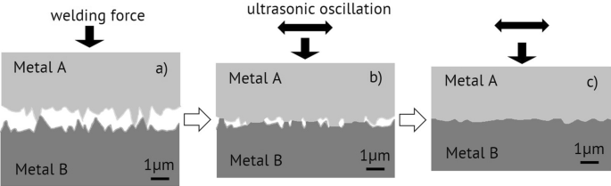

  

  Joining process of two metals. (a) The surfaces approximate due to the force applied by the sonotrode; (b) the US oscillation starts and flattens asperities as well as displaces contaminations and oxides from the joining area; (c) the juvenile surfaces contact and form adhesive bonds (Ref 44)

In conclusion, a physical metal bonding between the juvenile surfaces is mostly considered to be the main reason for the bond formation between the joining partners in US metal welding (Ref 10,11,12, 15, 17, 19, 21, 23,24,25,26). Mechanical interlocking was also observed to significantly contribute to the bond (Ref 10,11,12,13, 15, 17, 20), especially when the same materials are joined together, e.g., Al/Al joints (Ref 19).

The mechanical interlocking and the entailing deformations mainly occur directly in the interface line, as schematically displayed in Fig. 2 (Ref 10, 23). They are typically most pronounced in the region of highest pressure directly below the sonotrode tip (Ref 10). The interface between two metals remains macroscopically flat (Ref 10), but some studies observed that with increasing welding energy and increasing welding time wave-like structures were developing on a microscale (Ref 10, 27) since once developed microstructures can be destroyed again under continuing oscillation, which may lead to wave-like patterns (Ref 10). As mentioned before, an increase in induced energy—and thus a higher temperature—facilitates plastic deformation of the metals (Ref 10, 23, 28).

For the bond formation in metal/FRP joints, additional assumptions can be made: Because of the induced energy in the welding area, the thermoplastic matrix of the FRP fuses, which brings the fibers and the metallic joining partner closer together. Due to plastic deformation of the metal, fibers and metal can interlock, complemented by adhesive connection through the re-solidification of the matrix. The bond formation is shown schematically in Fig. 3 (Ref 6, 24, 29, 30). The joint strength increases significantly if interlocking between the joining partners is accomplished in the joining area (Ref 8, 31).

Fig. 3

Schematic microstructure of an US welded metal/FRP joint. (a) At the beginning of the process; (b) during the US oscillation, the thermoplastic matrix melts and causes approximation between fibers and metallic joining partner; (c) the bond is formed with adhesive forces and interlocking (Ref 6, 24, 29, 30)

The exact correlation between microstructure and mechanical properties of the US welded joints has not yet been fully understood (Ref 32). However, for the joining of metals, there have been approaches to quantify the correlation between the size of the interface area and the quality of the weld by means of the linear weld density. The linear weld density is defined by the ratio of bonded interface line and the length of the entire weld (Ref 25, 33).

In this work, FE-models of US welded joints were developed. Providing the required information about geometries and properties of the joints, interfaces of US welded joints were characterized, categorized and correlated to the achieved mechanical joint strength (Ref 25, 33), and the failure mechanism. For this purpose, favorable combinations of joining partners were selected and process parameters for defined levels of mechanical strength were identified and evaluated by tensile shear tests. For each level of mechanical strength, the samples were characterized considering fracture areas and micro sections of the interface. Based on the geometry of these characteristic areas, two-dimensional FE-models were created to analyze stress and strain distributions of the micro sections under external load.

2 Materials and Methods

2.1 Experimental Setup

Since their bond formation process is thought to be slightly different, metal/metal joints and metal/FRP joints were investigated separately. Hence, two representative hybrid material systems were considered in this work: Al/Cu joints with the materials EN AW-1050A and EN CW004A, representing a typical hybrid material system in electric industry and Al/GFRP joints with the materials EN AW-1050A and GF-PA6 (woven glass fiber textile 0/90° with 50% fiber volume content), representing lightweight constructions. This particular combination of the latter materials did not allow to expect high strength joints as known from other US welded metal/FRP joints, e.g., 97 MPa Ti6Al4V/CF-PEEK (Ref 6, 7). Since EN AW-1050A was known to be very deformable, it was expected to generate a higher diversity of interface characteristics. The thermoplastic matrix PA of the GFRP is well suited for USW due to its relatively low melting point of 220 °C (Ref 34) and finally, individual glass fibers are more visible by computer tomography (CT) than carbon fibers due to the greater difference of density between the fibers and the polymer matrix (Ref 35).

The mechanical properties of the joining materials, that were characterized by tensile tests using a TesT 50 kN, are represented in Table 1 along with the dimensions of the sheet material used in the welding experiments.

Table 1 Mechanical properties of materials and dimensions of the samples

For the Al/Cu joints, a roll seam welding unit Branson Ultraseam 20 with a rotatable sonotrode was used (Ref 36) and for the Al/GFRP joints, a torsional welding unit Telsonic TSP 3000 was used. The reason for this differing approach for the two material systems were a larger homogenous interface for the roll seam welding on the one hand for the metal/metal joints, and a better reproducibility of joint strengths for the metal/FRP joints using torsional welding on the other hand. A close-up of the sonotrodes during the welding processes is shown in Fig. 4(a) for roll seam welding, and in Fig. 4(c) for torsional welding, respectively. The joining partners are clamped with a force of 6 kN (roll seam welding) and 3.2 kN (torsional welding), respectively. To create the continuous roll seam the oscillating sonotrode rolls over the metal sheet (Fig. 4a), to create the circular weld it oscillates on its own axis (Fig. 4c). Figure 4(b) and (d) shows the respective sonotrode tips.

Fig. 4

(a) US roll seam welding setup; (b) close-up of the roll seam sonotrode tip; (c) torsional US welding setup; (d) close-up of the torsional sonotrode tip

To examine the relation between microstructure and mechanical strength, joints with differing bond qualities and mechanical strengths were produced. The goal was to create two tensile shear strength levels, termed X/X_low and X/X_high. The tensile shear strength ${\sigma }_{TS}$ of the joints was derived with tensile shear tests performed with a TesT 50 kN with a displacement-controlled setup of 0.05 mm/s.

2.2 Microstructural Characterization

To identify the interface characteristics in correlation to certain strength levels, several micro sections of the joints were prepared along defined paths as illustrated in Fig. 5. At least 3 sections were investigated in lateral and longitudinal direction for each Al/Cu sample and at least 5 sections were examined for each Al/GFRP sample. Only the interface located directly below the sonotrode tips was considered to be part of the weld seam/spot to ensure the comparability between same type of samples despite different welding parameters, even though bonding may not be limited to this area especially for the metal/FRP joints, as described in (Ref 31).

Fig. 5

(a) paths for micro sections for Al/Cu joints longitudinal and lateral to the weld seam; (b) paths for micro sections for Al/GFRP joints

The micro sections were investigated by light microscopy and scanning electron microscopy (SEM) to find characteristic traits, which were sized and used to characterize the weld quantitatively. Key aspects for the Al/Cu joints were the linear weld density, micro gaps, interlockings and large waves in the interface line, and the enlargement of the interface line due to overall waviness. Key aspects for the Al/GFRP joints were the proximity between fibers and metallic joining partner and the number and area of fibers directly connected with the metallic joining partner. Additionally, the shares of microsegments with the same characteristics for each weld seam/spot depending on the respective ${\sigma }_{TS}$ were determined.

In addition to the examination of the micro sections, fracture surfaces were investigated to verify the assumptions obtained from the analysis of the 2D-sections. The subject of interest was the linear weld density with respect to the complete joining area.

To examine the contact between the joining partners on a 3D-basis, including the interface geometry but also voids and proximity between fibers and metal, high-resolution x-ray CT-scans of Al/GFRP joints were performed on thin stripes of the samples to gain volume information. The CT-scans were conducted using a Zeiss Versa 520 with an accelerating voltage of 90 kV, a power density of 8 W, an exposure time of 5 s, and a resolution of 4.4 μm. The sample was rotated 360° and 2401 projections were acquired.

2.3 Development of FE-Models

The long-term goal of the presented research is to develop a contact model on component scale, which can simulate the behavior of an US welded joint using a simplified contact model including all relevant conditions that were derived from a realistic microscale model of the interface. Therefore, the influence of the geometry of the interface on the microscale needs to be investigated, to assure correct conclusions in future abstraction processes. This influence was examined by the following comparison between simplified and geometrically complex interfaces.

Basis for the microscale models were micro sections investigated by light microscopy (Al/Cu) and SEM (Al/GFRP), respectively. Sections which included specific interface characteristics were chosen for modeling. The obtained images were then transferred into FEM software using the procedure shown in Fig. 6. First, the microscopic image was transformed into a vector graphic with the aid of bitmap-tracing in the open-source software Inkscape by Inkscape Community (Fig. 6a and b). Based on this vector graphic, a 2D-surface model was created in Siemens Solid Edge ST9 (Fig. 6c), which was then imported into Simulia Abaqus 2021 by Dassault Systèmes to finalize the FE model (Fig. 6d).

Fig. 6

From micro section to FE-model. (a) Image from the light microscope (Al/Cu) and SEM (Al/GFRP); (b) vector graphic derived from the microscopic images with the aid of bitmap-tracing; (c) 2D-surface model in CAD-format based on the vector graphic; (d) complete FE-model with mesh

In Abaqus, the simulation was performed using a dynamic, implicit step. The material properties described in Table 1 were used for the Al/Cu joints, and for the Al-part of the Al/GFRP joints. The GFRP was split into the separate materials GF and PA with properties listed in Table 2.

Table 2 Material properties for modeling of Al/FRP microscale (Ref 34)

With these properties, an elastic-plastic material model was established. The plasticity was modeled as depicted in Fig. 7 with a trilinear progression of the stress over the strain (Ref 37). Note that due to the absence of a damage model for the single materials (Al, Cu, GF, PA), plastic strain exceeding the given elongation was permitted.

Fig. 7

Elastic-plastic material model used in the FE-simulation

A mesh with CPE4R element type was used for quadratic elements and a CPE3 element type for triangular elements. The meshing in the Al/Cu model was done with quad-dominated elements with an approximate average element size of 2 µm in the interface line and 5 µm in the rest of the geometry, which added up to a total of approximately 1 × 10⁴ elements, with permission for the number of elements to increase or to decrease when appropriate during the meshing with respect to angles and radii. The maximum deviation factor for the elements was given by 0.1. The same element types and deviation factors were applied in the Al/GFRP joints, but, due to the difference in model size, the edge length of the elements in the interface was set to 0.5 µm, 1 µm between fibers and matrix and 2 µm in the rest of the geometry, which lead to a sum of 2.4 × 10⁴ elements. The meshes around the interface line are illustrated in Fig. 8(d) and (e).

Fig. 8

Interfaces, displacement, and mesh of the models. (a) Highlighted interface line with cohesive behavior for Al/Cu joints; (b) highlighted interface line with cohesive behavior for Al/GFRP joints; (c) sketch of the support structure, the boundary conditions and applied outer displacement; (d) mesh around the interface line of the Al/Cu joint; (e) mesh around the interface line of an Al/GFRP joint

Additional support structures were built around the original geometries, as displayed by the hatched areas in Fig. 8(c). These support structures had the same material properties as the original geometry they surrounded, presented in Table 1. For the discussion of the results, those support geometries were neglected since they were not of interest but transmitted the external loading to the interface.

The external loading was modeled as a displacement to simulate the tensile shear test from the experiments. For this purpose, the lower edge of the support structure of the lower joining partner was fixed with an encastre condition, and the upper edge of the support structure of the upper joining partner was moved with a uniform displacement in the x-direction, as presented in Fig. 8(c). The magnitude of the displacements of the upper edge for these microscale models were determined based on the tensile shear tests. Including the support structures, the Al/Cu joints had a total width of 300 µm and the Al/GFRP joints measured 90 µm.

The contact conditions were implemented as surface-to-surface interaction between the two parts Cu and Al as illustrated by the black line in Fig. 8(a). For the Al/GFRP joints, the location of the cohesive interface changed between Al-GF and Al-PA as illustrated by the black line in Fig. 8(b). The glass fibers were fixed in the matrix with a tied constraint to avoid potential delamination.

In this approach, a cohesive zone model, which included a damage model for the joints similar to models focusing on interface damages and delamination of composites (Ref 38,39,40,41,42), was used for the interactions between the joining partners. The basis for cohesive contact is a bilinear cohesive law with an elastic traction-separation behavior, which is mathematically expressed for two-dimensional calculations before damage initiation by Eq. (1) (Ref 37):

$$\left[ {\begin{array}{*{20}c} {T_{n} } \\ {T_{s} } \\ \end{array} } \right] = \left[ {\begin{array}{*{20}c} {K_{nn} } & {K_{ns} } \\ {K_{ns} } & {K_{ss} } \\ \end{array} } \right] \left[ {\begin{array}{*{20}c} {\delta_{n} } \\ {\delta_{s} } \\ \end{array} } \right]$$

(1)

K is the contact stiffness, δ the displacement between two corresponding points at the interface, T_n and T_s are the normal and shear traction, the indices n and s represent the two loading directions. In a surface-based cohesive model, the traction is defined as the ratio between the contact force and the current area at each contact point. In the chosen uncoupled traction-separation behavior, only K_nn and K_ss need to be specified since pure normal separation does not produce cohesive forces in the shear directions and vice versa. Assuming isotropic behavior, the parameters K_nn and K_ss have the same values and will therefore be written as K_eff (Ref 37, 39).

The maximum nominal stress criterion was used for damage initiation, which is defined by Eq. (2) and translates into the maximal traction for surface-based cohesive zone modeling. T_n⁰ and T_s⁰ are input values which represent the highest contact stresses. In an isotropic case, they have the same value and can therefore be written as the damage initiation traction Tm (Ref 37). Note that by using another criterion, damage initiation could also be defined by specifying the separation instead of the traction.

$$\max \left\{ {\frac{{\left\langle {T_{n} } \right\rangle }}{{T_{n}^{0} }},\frac{{T_{s} }}{{T_{s}^{0} }}} \right\} = \max \left\{ {\frac{{\left\langle {T_{n} } \right\rangle }}{{T_{m} }},\frac{{T_{s} }}{{T_{m} }}} \right\} = 1$$

(2)

Damage evolution must be specified if visible separation of the created bond is desired after damage initiation, which is advantageous for reasons of visual presentation and analysis in this case. This is possible by giving the fracture energy G_c or the plastic displacement δ_pl and a linear, exponential, or tabular form of softening. With a linear softening and an isotropic behavior, which is permissible due to the two-dimensional nature of the geometrical model, the traction-separation behavior can be depicted like in Fig. 8 (Ref 37).

Thus, to define the behavior of the interfaces using Abaqus, the traction at the point of damage initiation in any direction Tm, the stiffness K_eff and the critical fracture energy G_c or, alternatively, the plastic displacement δ_pl need to be specified. G_c is calculated as the area under the triangle in Fig. 9 and K_eff constitutes the slope until the point of damage initiation.

Fig. 9

Bilinear traction-separation behavior for cohesive zone models (Ref 37)

Since there was no pre-existing contact model specifically for US welded joints, the values for the mentioned contact parameters were unknown. In previous research, US welded joints were modeled on component scale, (Ref 31, 43), but not on microscale. So, in this approach, values of K_eff and δ_pl were inspired by literature calculations for cohesive zone models (Ref 40) and kept constant with K_eff = 100,000 MPa/µm and δ_pl = 0.005 µm. Only the damage initiation traction Tm was varied.

To understand the influence of different damage initiation tractions, reference simulations with flat interface geometries were performed. The flat interface geometry is easy to model, does not require knowledge about the exact interface composition and is consequently most user-friendly. With the help of those reference simulations, it was possible to determine to what extent the behavior of such a simplified model already matched that of a model with a real interface geometry only due to the same contact conditions. The flat-interfaced geometries, termed simplified geometries, also represent the long-term pursued component scale models, and were modeled with the same material properties, the same outer dimensions, and the same external displacements as the models with more complex interface geometries, termed real geometries. The reference simulations were run to find the highest damage initiation traction Tm₁ where the interface completely failed, and the lowest damage initiation traction Tm₂ > Tm₁ where the interface remained completely intact during the simulations (Fig. 10a). The limits Tm₁ and Tm₂ are crucial for an accurate description of the actual behavior of a bond under this specific displacement for a given geometry.

Fig. 10

Implementation of damage initiation tractions Tm which lead to different failure modes of the interfaces at a given displacement. (a) Reference model with flat, simplified interface geometry. Damage initiation traction Tm₁ leads to failure of the interface while damage initiation traction Tm₂ leaves it intact; (b) model with real, complex interface. Damage initiation traction Tm₁^′ leads to failure of the interface while damage initation traction Tm₂^′ leaves it intact

Tm₁ and Tm₂ were then used as initial damage initiation tractions for the real models. In cases where Tm₁ and Tm₂ were not the limits between failed and intact interface, they were adjusted to Tm₁^′ and Tm₂^′ (Fig. 10b), with Tm₁^′ marking the highest damage initiation traction for a completely failed interface and Tm₂^′ marking the lowest damage initiation traction for a completely intact interface for the real geometries. The difference between Tm₁, Tm₂ and Tm₁^′, Tm₂^′ represents the influence of the interface geometry and gives further information for the development of a contact model.

The components of the stress response in x-direction (Sxx), i.e., the direction of the displacement, as well as the deformations and the strain in x-direction (Exx) for the reference simulation are displayed for Tm ≤ Tm₁ (failed interface) in Fig. 11(a), (c), (e), (g) and Tm ≥ Tm₂ (intact interface) in Fig. 11(b), (d), (f), (h). Their distribution is used to establish a foundation for the understanding of the results of the real simulations.

Fig. 11

Strain and stress in x-directions Exx and Sxx of reference simulations with simplified geometries. (a) Exx for Al/Cu joints with failed interface; (b) Exx for Al/Cu joints with intact interface; (c) Sxx for Al/Cu joints with failed interface; (d) Sxx for Al/Cu joints with intact interface; (e) Exx for Al/GFRP joints with failed interface; (f) Exx for Al/GFRP joints with intact interface; (g) Sxx for Al/GFRP joints with failed interface; (h) Sxx for Al/GFRP joints with intact interface. Deformation factor for Al/Cu joints = 25, deformation factor for Al/GFRP joints = 50

As expected, no stress and small plastic strain remained in the simplified geometries after failure for the reference simulation. Without interface failure, on the other hand, strain and stress in the peripheral areas of the geometry and the interface were most prominent.

The results of the calculations both for the displacement of the upper edge and the damage initiation tractions Tm₁ and Tm₂ are shown in Table 3.

Table 3 Displacement calculated from tensile shear tests with damage initiation tractions Tm₁ and Tm₂ where change in interface failure was to be expected as from the reference simulations

3 Results

3.1 Welding experiments

3.1.1 Al/Cu joints

3.1.1.1 Tensile Shear Strength σ _TS

To produce joints with different bond qualities, i.e., different σ_TS, preliminary tests were performed to identify suitable parameter sets. Aim of this part of the study was to find a combination of amplitude u, velocity of the sonotrode v and welding force F that repeatedly produced varying σ_TS by maintaining two of the three parameters and varying the third. This was done with regard to the following analysis of the microstructure to determine the influence of one parameter. For the Al/Cu joints, the preliminary experiments indicated that it was effective to maintain u and v. Several series of tests were then performed with varying welding forces F. In most of the investigated cases, there was a noticeable trend of increasing σ_TS with increasing F, and sometimes even a change in the failure mode (interfacial failure or failure of the aluminum) depending on that parameter.

To identify the characteristics of the microstructures, different levels of σ_TS were generated by certain parameter sets achieved in the preliminary parameter studies. The parameters u = 25 µm, v = 10 mm/s, F = 200 N, which lead to an average σ_TS = 4 MPa, were then chosen for the set with low σ_TS, termed Al/Cu_low. For the set with high σ_TS, termed Al/Cu_high, the parameters u = 25 µm, v = 10 mm/s, F = 300 N (average σ_TS = 16 MPa) were chosen. The parameter set Al/Cu_comp with u = 16 µm, v = 2 mm/s, F = 150 N (average σ_TS = 12 MPa) was also investigated and characterized for additional comparison. This very different parameter set resulted in a comparable total energy input, which is the defining factor for bond formation, and in a comparable level of σ_TS, consequently allowing this investigation.

3.1.1.2 Investigations of the Interface Via Micro Sections

As discussed in Sect. 2.2, the focus of the interface analysis of the Al/Cu joints was on the linear weld density, the micro gaps, and the waves in the interface. This led to three key categories observable in the interface characterization. These categories, shown in Fig. 12, were:

• (a) no contact between the two joining partners

• (b) overall contact between the joining partners, but several micro gaps between Al and Cu in the interface line

• (c) direct contact between the joining partners with a wavy interface

Fig. 12

Interface line for Al/Cu joints with different characteristics: (a) category a; (b) category b; (c) category c

Each segment of the micro section was assigned to one of the categories and the relative proportions for each category were compared. Figure 13 shows the shares each category had in the weld seam for the three different parameter sets Al/Cu_low, Al/Cu_high and Al/Cu_comp. For all three parameter sets, the unbonded regions, category a, constituted the majority of the joining area, but the two sets Al/Cu_high and Al/Cu_comp which had a higher σ_TS, also contained larger shares of category c.

Fig. 13

Shares in the weld seam with characteristics of the microstructure specified in Fig. 12. (a) Al/Cu_low (typical σ_TS = 4 MPa); (b) Al/Cu_high (typical σ_TS = 16 MPa); (c) Al/Cu_comp (typical σ_TS = 12 MPa)

Further information about the Al/Cu interfaces is given in Table 4 considering the direction of the investigated sections and more information regarding the individual characteristics. As mentioned above, the ratio between the length of the bonded interface line and the total interface line constitutes the linear weld density. The difference in the linear weld density was striking between the joints with lower (Al/Cu_low) and higher (Al/Cu_high and Al/Cu_comp) σ_TS, (see Fig. 13) indicating an overall larger bonded area for bonds with higher σ_TS, as expected from the bond formation theories discussed in Sect. 1, and confirmed by the investigations of the fracture surfaces, discussed in the next section.

Table 4 Characteristics of the interface lines for Al/Cu joints

Category b and category c both contribute to the bonded region but show very different interface geometries which are worth further analysis. The detailed quantity and length of the micro gaps (category b) is also listed in Table 4. The difference in gap lengths between the considered parameter sets was relatively small, but the Al/Cu_low joints, i.e., the joints with the lowest σ_TS, contained most gaps per mm, which also is in accordance with the abovementioned bond formation theory.

The wavy interface (category c) was characterized in two ways: first, the general waviness and the resulting extension of the interface line by 1.2–6.6% and secondly, the dimensions of larger waves > 1 µm that were expected to support the joint strength by interlocking, (see Fig. 12c). Both Al/Cu_high and Al/Cu_comp joints featured major waves in their interfaces with a length up to 40 µm and height up to and 6–8 µm, while Al/Cu_low joints did not show any waves > 1 µm. In previous research, the mechanical interlocking of the materials was often cited as an important contributor to the formation of the bond or its mechanical strength (Ref 10, 27). Since the joints with higher σ_TS featured more major waves in the presented investigation as well, the same could be concluded here.

3.1.1.3 Fracture Surfaces

Fracture surfaces from the tensile shear tests were investigated under the light microscope. As shown exemplarily in Fig. 14(a) and (b), the edges of the bonded region are marked by the red line. It was possible to determine the percentage of the bonded area with respect to the entire joining area for the investigated strength levels, correlating to the linear weld density determined in the analysis of the micro sections (Table 4). Figure 14(c) shows the rising relation between welding force and bonded area for parameter sets with constant amplitude and sonotrode velocity. The parameters investigated here were Al/Cu_low and Al/Cu_high as well as two additional parameter combinations with the same amplitude and sonotrode velocity u = 25 µm, v = 10 mm/s, F = 150 N and u = 25 μm, v = 10 mm/s, F = 250 N.

Fig. 14

(a) Fracture surface of Cu-side for an Al/Cu_low joint (parameter set u = 25 µm, v = 10 mm/s, F = 200 N, typical σ_TS = 4 MPa); (b) fracture surface for Cu-side for an Al/Cu_high joint (parameter set u = 25 µm, v = 10 mm/s, F = 300 N, typical σ_TS = 16 MPa); (c) bonded area for Al/Cu joints depending on the welding force (parameter set u = 25 µm, v = 10 mm/s, F = 150, 200, 250, 300 N)

3.1.2 Al/GFRP Joints

3.1.2.1 Tensile shear strength σ _TS

Analogous to the Al/Cu joints, Al/GFRP joints with specific σ_TS levels were generated. Al/GFRP_low joints with σ_TS = 1.6 MPa were manufactured with an amplitude u = 55 µm, an energy E = 700 Ws, and a pressure p = 1 bar, while Al/GFRP_high joints with σ_TS = 6 MPa were manufactured with u = 55 µm, E = 700 Ws, p = 0.5 bar. Also, joints Al/GFRP_comp with σ_TS = 5 MPa were produced with u = 55 µm, E = 500 Ws, p = 0.5 bar.

3.1.2.2 Investigation of the Interface Microstructure Via Micro Sections

As explained in Sect. 1, the bond formation of metal/FRP joints is heavily influenced by the proximity and interlocking of the fibers and the metallic joining partner. From previous research (Ref 31) it is also known that close proximity or even interlocking between fibers and metallic joining partners is associated with higher local shear strengths in torsional US joints. The interfaces were categorized by five characteristics, shown in Fig. 15:

• (a) flat interface line with contact only between polymer matrix and aluminum, large space between fibers and aluminum

• (b) deformation of both aluminum and polymer matrix by welding

• (c) flat interface line with contact between matrix and aluminum, with approximation of fibers to aluminum

• (d) direct contact between fibers and aluminum

• (e) interlocking between fibers and aluminum

Fig. 15

Interface line for Al/GFRP joints with different forms of bonding. (a) Category a; (b) category b; (c) category c; (d) category d; (e) category e

Each segment of the micro sections was assigned to one of the categories and the relative proportions for each category were compared. Figure 16 shows the shares each category had in the weld spot for the three different parameter sets Al/GFRP_low, Al/GFRP_high and Al/GFRP_comp.

Fig. 16

Shares in the interfaces with characteristics of the microstructure specified in Fig. 15. (a) Al/GFRP_low (typical σ_TS = 1.6 MPa); (b) Al/GFRP_high (typical σ_TS = 6 MPa); (c) Al/GFRP_comp (typical σ_TS = 5 MPa)

Apparently, category a was by far the most prominent type of bonding in all investigated joints, but especially for the Al/GFRP_low joints, where it made up more than 75% of the weld area. For Al/GFRP_high and Al/GFRP_comp, the share of category b constituted the greatest difference, whereas the percentages of categories c-e were comparable over all three parameter sets, even though there is a trend of a higher percentage of category d and e in bonds with higher σ_TS.

The investigation of fracture surfaces with correlation to the linear weld density and strength level of the joints was not effective for the Al/GFRP joints. Due to the melting of the PA matrix, the determination of the bonded area was associated with high uncertainties. Another factor was, that the proximity between fibers and metallic joining partner, which is the essential for the analysis for metal/FRP joints, as illustrated by Fig. 15, cannot be analyzed in a non-destructive way over the whole area of the fracture surfaces. Therefore, CT-scans and the analysis of microsections are a more suitable way to describe the total interface of an Al/GFRP joint with respect to the whole bond area.

3.1.2.3 CT-scans

CT-scans allowed to examine the characteristics of the bonding area between the two joining partners on a three-dimensional basis over the entire joining area. This completed the classification of the contact between fibers and metal in case of the Al/GFRP joints. Figure 17 shows six layers of an Al/GFRP joint with a distance in the z-direction of 0.4 mm between each of them. The white reticle marks the same x–y position on all layers for orientation. The fibers on the right sides of the images are shown in a front view (cross section) and the fibers on the left sides are shown in a side view, so the bonding between fiber and metal can be viewed from both possible angles in accordance with the orientations of the fabric in 0° and 90°. Figure 17 shows how the Al adapted to the undulation through plastic deformation. Additionally, a clear connection between fibers and aluminum is visible on all six layers over the distance of 2 mm, especially in the region circled in Fig. 17. This verifies the successful interlocking between fibers and metal in the whole joining area. Therefore, the 2D FE-model of the interface region in this work can be considered as representative for the whole joining area. Besides the verification of successful welding processes, more detailed CT-scans will provide data for 3D FE-models.

Fig. 17

CT-scan projection of the same xy-positions, indicated by the white reticle, of an Al/GFRP joint. (a) at 3.43 mm scan depth; (b) 3.03 mm scan depth; (c) 2.63 mm scan depth; (d) 2.23 mm scan depth; (e) 1.83 mm scan depth; (f) 1.43 mm scan depth in z-direction, measured from the edge of the sample

3.2 FE-Simulations of Microsegments

3.2.1 Al/Cu Joints

The geometry of the Al/Cu joint considered for simulation on the microscale features a major wave with a fully bonded interface and can be assigned to category c. Before discussing the distribution of strain and stress for failed and intact interfaces under loading, the new values Tm₁^′ and Tm₂^′ needed to be determined. For this, Tm₁ and Tm₂ from the reference simulations served as starting values. To assess whether the interface of the real models failed under the given external load, the output value status of the cohesive contact (CSTATUS) under the simulated conditions (Ref 37) was evaluated. Figure 18 shows the status of the bond for the Al/Cu joint depending on the used Tm. It becomes apparent that the values Tm₁^′ for a completely failed interface and Tm₂^′ for an intact interface were quite far apart from each other, and that the transition between the two states contained more intermediate states than was the case in the reference simulations. The influence of the wave in the geometry on damage initiation is well illustrated through these intermediate states.

Fig. 18

Evolution of the status of the bond from failing to intact interface depending on damage initiation traction Tm for the Al/Cu joint. (a) Tm = Tm₁^′ = 64 MPa; (b) Tm = 90 MPa; (c) Tm = 100 MPa; (d) Tm = 110 MPa; (e) Tm = 125 MPa; (f) Tm = Tm₂.^′ = 174 MPa. Deformation scale factor = 2

Figure 19 shows Exx and Sxx for Tm ≤ Tm₁^′, (failed interface) and Tm ≥ Tm₂^′ (intact interface). In Fig. 19(a) and (b), the applied displacement of 1.2 µm (0.4% strain), caused the failure of the joint for Tm ≤ Tm₁^′. Strain mostly occurred in the softer Al component of the joint and predominantly in the inner part of the major wave as the wave started shearing off after joint failure, accompanied by compressive stress in the affected regions. The interlocking by the wave could absorb the force induced by the displacement, indicated by the resulting stress and strain and confirming the theory of increasing joint strength due to plastic deformation and interlocking of the joining partners.

Fig. 19

Local strain and stress distribution in x-directions $Exx$ and Sxx for the microscale model of an Al/Cu joint. (a) Exx for a failed interface with Tm ≤ Tm₁^′; (b) Sxx for a failed interface with Tm ≤ Tm₁^′; (c) Exx for an intact interface with Tm ≤ Tm₂^′; (d) Sxx for an intact interface with Tm ≤ Tm₂.^′. Deformation scale factor = 10

In Fig. 19(c) and (d), for Tm ≥ Tm₂^′, the joint remained intact. Like in the reference simulations (Fig. 11), this resulted in strain in the peripheral zones of the interface line, but strain in the immediate vicinity of the large wave is also visible.

Table 5 shows the resulting limits of the damage initiation tractions Tm₁^′ and Tm₂^′ for the Al/Cu joint. The difference between Tm_1,2 and Tm_1,2^′ marks the influence of the interface geometry on the behavior of the joint and is an indicator for the alignment from microscale models to component scale models.

Table 5 Damage initiation stresses for failing and intact bonding contact in the interface under the given displacement for the real Al/Cu joint

3.2.2 Al/GFRP Joints

Models of the interface geometry categories c (flat interface line with contact between matrix and aluminum, with approximation of fibers to aluminum) and e (interlocking between fibers and aluminum) are discussed in the following since they represent variations with and without direct contact between fibers and metallic joining partner. The new values Tm₁^′ and Tm₂^′ were determined analogously to the analysis of the Al/Cu joints. Figure 20 shows the status of the bond for the Al/GFRP joint category e depending on the used damage initiation traction.

Fig. 20

Evolution of the status of the bond from failing to intact interface depending on damage initiation traction for Al/GFRP category e joint (a) Tm = Tm₁^′ = 3 MPa; (b) Tm = 5 MPa; (c) Tm = 6 MPa; (d) Tm = 7 MPa; (e) Tm = Tm₂.^′ = 8 MPa. Deformation factor = 20

Figure 21 shows Exx and Sxx for Tm ≤ Tm₁^′, (failed joint) and Tm ≥ Tm₂^′ (intact joint) for both categories c and e. In Fig. 21(a), (c), (e) and (g), the applied displacement of 0.14 µm (0.15% strain), caused failure for Tm ≤ Tm₁^′.

Fig. 21

Local strain and stress in x-directions Exx and Sxx for microscale models category c and category e of Al/GFRP joints. (a) Exx for a failed interface with Tm ≤ Tm₁^′ for category c; (b) Exx for an intact interface with Tm ≥ Tm₂^′ for category c; (c) Sxx for a failed interface with Tm ≤ Tm₁^′ for category c; (d) Sxx for an intact interface with Tm ≥ Tm₂^′ for category c; (e) Exx for a failed interface with Tm ≤ Tm₁^′ for category e; (f) Exx for an intact interface with Tm ≥ Tm₂^′ for category e; (g) Sxx for a failed interface with Tm ≤ Tm₁^′ for category e; (h) Sxx for an intact interface with Tm ≥ Tm₂.^′ for category e. Deformation scale factor = 50

Considering category c in case of failure (Fig. 21a), compressive and tensile strain occurred in the PA matrix close to the interface line due to the stiffer aluminum moving over the PA surface while shearing off the PA surface roughness. In contrast for the intact joint (Fig. 21b), strain occurred in higher intensity around the glass fibers since Tm₂^′ was exceeded the interface remained intact and the deformation was completely transferred to the softest material in the system, the PA matrix. In both cases the strain was accompanied by appropriate compressive and tensile stresses in the affected areas (Fig. 21c and d).

Similar effects were observed in the model of category e. In case of failure, (Fig. 21e) small strain occurred in the aluminum close to the interface line due to shearing. However, in this case, the deformation was also transferred to the PA matrix, indicating an absorption of force and hence, confirming the effect of interlocking with respect to higher joint strength. Additionally, the higher resulting stress close to the interface between aluminum and glass fibers (Fig. 21g) in comparison to the joints with a PA interlayer (category c Fig. 21c), indicates a higher capability of force absorption under load for joints with metal/fiber interlocking.

In the intact joint of category e (Fig. 21f) the same force acted as in category c, but in contrast to category c there was no soft PA interlayer to absorb it by deformation, resulting in low strains but higher stress in the interface (Fig. 21h). Table 6 shows an overview of the limits Tm₁^′ and Tm₂^′ for the displacement associated with the Al/GFRP joints for both categories c and e. The comparison shows that Tm_1,2 and Tm_1,2^′ differed by a significant percentage in most cases, which is to be factored in for the further development of the contact model on component scale. Note that the reference simulations for the Al/GFRP joints were run with solely PA because the glass fibers in the real models were arranged orthogonally to the load direction.

Table 6 Damage initiation tractions for failing and intact bonding contact in the interface under the given displacement for Al/GFRP joints

4 Summary, Conclusions and Outlook

To develop a reliable FE model for US welded joints, samples with clearly differing levels of strength were generated for combinations of Al/Cu and Al/GF-PA to correlate relevant interface characteristics with the resulting joint strength. Higher and lower tensile shear strengths σ_TS were achieved by an appropriate choice of the USW parameters. Al/Cu joints manufactured in an US roll seam welding process with σ_TS = 4 MPa and σ_TS = 16 MPa and Al/GFRP joints manufactured in a torsional welding process with σ_TS = 1.6 MPa and σ_TS = 6 MPa were investigated. Microstructural characteristics were categorized, quantified, and successfully correlated to σ_TS including linear weld density, micro gaps and mechanical interlockings.

As expected, larger linear weld densities, fewer micro gaps, and mechanical interlocking lead to higher joint strengths.

Microscopic FE-models were created by importing images from light microscopy and SEM including geometrical details of the interface. Tensile shear tests of the US welded joints provided information about the macroscale deformation behavior that was implemented in the simulations. Damage initiation traction was iteratively determined considering the bond status under load.

The simulations of joints under tensile shear load showed reasonable distributions of strains and stresses supporting common theories with respect to the correlation of interlocking with higher joint strength.

Finally, factors to implement the findings of this work in a simplified geometry that could be used for component scale models were determined for all joints investigated. However, a realistic model requires a holistic characterization of the joints, including relevant multiaxial load scenarios (e.g., tension, compression, shearing, bending, torsion) and realistic ambient conditions (e.g., temperature or environmental media). Also, the effect of the different directions of the oscillations in the various USW technologies on the geometry of the interface on the microscale presents a topic for future investigations.

In conclusion, the main aspects of the study were:

• (1) Categorisation and quantification of interface characteristics with correlation to the joint strength.

• (2) Transmission from microscopy images to FEM including the determined interface characteristics.

• (3) Development of a microscale contact model for US welded multi-material joints

• (4) Simulation of resulting stress and strain distribution at and close to the interface under tensile shear load, supporting common theories with respect to the correlation of interlocking with higher joint strength.

References

F. Balle, G. Wagner, and D. Eifler, Ultrasonic Spot Welding of Aluminum Sheet/Carbon Fiber Reinforced Polymer - Joints, Mat.-Wiss. U. Werkstofftech., 2007 https://doi.org/10.1002/mawe.200700212
M.P. Matheny and K.F. Graff, Ultrasonic Welding of Metals, 2015
S. Elangovan, S. Semeer, and K. Prakasan, Temperature and Stress Distribution in Ultrasonic Metal Welding—An FEA-Based Study, J. Mater. Process. Technol., 2009 https://doi.org/10.1016/j.jmatprotec.2008.03.032
G. Wagner, F. Balle, and D. Eifler, Ultrasonic Welding of Hybrid Joints, JOM, 2012 https://doi.org/10.1007/s11837-012-0269-5
F. Balle, G. Wagner, and D. Eifler, Ultrasonic Metal Welding of Aluminium Sheets to Carbon Fibre Reinforced Thermoplastic Composites, Adv. Eng. Mater., 2009 https://doi.org/10.1002/adem.200800271
M. Liesegang, S. Arweiler, T. Beck, and F. Balle, Orbital Ultrasonic Welding of Ti-Fittings to CFRP-Tubes, JMMP, 2021 https://doi.org/10.3390/jmmp5020030
M. Liesegang, Kontinuierliches Ultraschallschweißen ebener und rohrförmiger Titan/CFK-Verbindungen - sonotroden, Prozessentwicklung und Verbundeigenschaften, Dissertation, Technische Universität Kaiserslautern, Kaiserslautern, 2020
F. Balle, Ultraschallschweißen von Metall/C-Faser-Kunststoff (CFK)-Verbunden, Dissertation, Technische Universität Kaiserslautern, Kaiserslautern, 2009
M. Jung and U. Langer, Methode der finiten Elemente für Ingenieure: Eine Einführung in die numerischen Grundlagen und Computersimulation, 2nd ed. Springer, Wiesbaden, 2013.
D. Bakavos and P.B. Prangnell, Mechanisms of Joint and Microstructure Formation in High Power Ultrasonic Spot Welding 6111 Aluminium Automotive Sheet, Mater. Sci. Eng. A, 2010 https://doi.org/10.1016/j.msea.2010.06.038
E. de Vries, Mechanics and Mechanisms of Ultrasonic Metal Welding, The Ohio State University, Ohio, 2004.
J. Wodara, Das Ultraschall-Punktschweißen metallischer Werkstoffe, Dissertation, TH Otto von Guericke Magdeburg, Magdeburg, 1984
J. Magin, Ultraschalltorsionsschweißen von Aluminium/Titan-Verbunden-Prozessanalyse, mechanische Eigenschaften und Mikrostruktur, Dissertation, Technische Universität Kaiserslautern, Kaiserslautern, 2015
N. Shen, A. Samanta, H. Ding, and W. Cai, Simulating Microstructure Evolution of Battery Tabs During Ultrasonic Welding, J. Manuf. Process., 2016, 5, p 306–314.
J. Wodara, Ultraschallfügen und -trennen, Verlag für Schweißen und verwandte Verfahren DVS-Verlag GmbH, Düsseldorf, 2004.
C. Doumanidis and Y. Gao, Mechanical Modeling of Ultrasonic Welding: Analytical and Numerical Modeling of Spot Ultrasonic Welding on Thin Metal Foils is Motivated by a New Ultrasonic Rapid Prototyping Technology, Springer, Berlin, 2004.
J. Wodara, Verbindungsbildung Beim Ultraschallschweissen Metallischer Werkstoffe, ZIS-Mitteilungen, 1986, 28(1), p 102–108.
H. Li, H. Choi, C. Ma, J. Zhao, H. Jiang, W.C. Abell, and J.A.L. Xiaochun, Transient Temperature and Heat Flux Measurement in Ultrasonic Joining of Battery Tabs Using Thin-Film Microsensors, J Manuf Sci Eng, 2013, 135(5), p 478.
X. Wu, T. Liu, and W. Cai, Microstructure, Welding Mechanism, and Failure of Al/Cu Ultrasonic Welds, J. Manuf. Process., 2015 https://doi.org/10.1016/j.jmapro.2015.06.002
R.A. Behnagh, P. Esmaeilzadeh, and M.A.M. Pour, Simulation of Ultrasonic Welding of Al-Cu Dissimilar Metals for Battery Joining, Adv. Des. Manuf. Technol., 2020, 13(2), p 23–31.
A. Siddiq and E. Ghassemieh, Thermomechanical Analyses of Ultrasonic Welding Process Using Thermal and Acoustic Softening Effects, Mech. Mater., 2008 https://doi.org/10.1016/j.mechmat.2008.06.004
Y.Y. Zhao, D. Li, and Y.S. Zhang, Effect of Welding Energy on Interface Zone of Al-Cu Ultrasonic Welded Joint, Sci. Technol. Weld. Join., 2013, 18(4), p 354–360.
J. Harthoorn, Ultrasonic metal welding, Dissertation, De Technische Hogeschool Eindhoven, Niederlande, 1978
Z.S. Al-Sarraf, A study of ultrasonic metal welding, PhD thesis, University of Glasgow, Glasgow, 2013
S. Dhara and A. Das, Impact of Ultrasonic Welding on Multi-Layered Al–Cu Joint for Electric Vehicle Battery Applications: A Layer-Wise Microstructural Analysis, Mater. Sci. Eng. A, 2020 https://doi.org/10.1016/j.msea.2020.139795
G. Baladin, V.A. Kuznetsov, and L. Silin, Fretting Action Between Members in the Ultrasonic Welding of Metals, Weld. Prod., 1967, 10, p 77–80.
R. Jahn, R. Cooper, and D. Wilkosz, The Effect of Anvil Geometry and Welding Energy on Microstructures in Ultrasonic Spot Welds of AA6111-T4, Metall. Mater. Trans. A, 2007 https://doi.org/10.1007/s11661-006-9087-0
F. Haddadi and D. Tsivoulas, Grain Structure, Texture and Mechanical Property Evolution of Automotive Aluminium Sheet During High Power Ultrasonic Welding, Mater. Charact., 2016 https://doi.org/10.1016/j.matchar.2016.06.004
F. Staab, F. Balle, and J. Born, Ultrasonic Torsion Welding of Aging Resistant Al/CFRP Joints - Concepts, Mechanical and Microstructural Properties, KEM, 2017 https://doi.org/10.4028/www.scientific.net/KEM.742.395
G. Wagner, F. Balle, and D. Eifler, Ultrasonic Welding of Aluminum Alloys to Fiber Reinforced Polymers, Adv. Eng. Mater., 2013 https://doi.org/10.1002/adem.201300043
F. Staab, M. Liesegang, and F. Balle, Local Shear Strength Distribution of Ultrasonically Welded Hybrid ALUMINIUM to CFRP Joints, Compos. Struct., 2020 https://doi.org/10.1016/j.compstruct.2020.112481
H.T. Fujii, Y. Goto, Y.S. Sato, and H. Kokawa, Microstructure and Lap Shear Strength of the Weld Interface in Ultrasonic Welding of Al Alloy to Stainless Steel, Scripta Mater., 2016 https://doi.org/10.1016/j.scriptamat.2016.02.004
C.Y. Kong, R.C. Soar, and P.M. Dickens, Characterisation of Aluminium Alloy 6061 for the Ultrasonic Consolidation Process, Mater. Sci. Eng. A, 2003 https://doi.org/10.1016/S0921-5093(03)00590-2
ANSYS Inc., Cambridge, UK, Ansys GRANTA EduPack software, 2020 (www.ansys.com/materials)
J. Kastner, E. Schlothauer, P. Burgholzer, and D. Stifter, Comparison of x-ray computed tomography and optical coherence tomography for characterisation of glass-fibre polymer matrix composites, in Proceedings of World Conference on Non Destructive Testing, 2004, pp. 71–79
M. Liesegang, Y. Yu, T. Beck, and F. Balle, Sonotrodes for Ultrasonic Welding of Titanium/CFRP-Joints—Materials Selection and Design, JMMP, 2021 https://doi.org/10.3390/jmmp5020061
Dassault Systèmes Simulia Corp., Abaqus Theory Manual, Dassault Systèmes Simulia Corp., 2021
A. Ali, A. Lo Conte, C.A. Biffi, and A. Tuissi, Cohesive Surface Model for Delamination and Dynamic Behavior of Hybrid Composite with SMA-GFRP Interface, Int. J. Lightweight Mater. Manuf., 2019 https://doi.org/10.1016/j.ijlmm.2019.01.006
M. Ramamurthi and Y.S. Kim, Delamination Characterization of Bonded Interface Using Surface Based Cohesive Model, Int. J. Precis. Eng. Manuf., 2013 https://doi.org/10.1002/9781118356074.ch38
A. Turon, C.G. Dávila, P.P. Camanho, and J. Costa, An Engineering Solution for Mesh Size Effects in the Simulation of Delamination Using Cohesive Zone Models, Eng. Fract. Mech., 2007 https://doi.org/10.1016/j.engfracmech.2006.08.025
Z. Zou and M. Hameed, Combining Interface Damage and Friction in Cohesive Interface Models Using an Energy Based Approach, Compos. A Appl. Sci. Manuf., 2018 https://doi.org/10.1016/j.compositesa.2018.06.017
B. Benamar, M. Mokhtari, K. Madani, and H. Benzaama, Using a Cohesive Zone Modeling to Predict the Compressive and Tensile Behavior on the Failure Load of Single Lap Bonded Joint, Frattura ed Integrità Strutturale, 2019 https://doi.org/10.3221/IGF-ESIS.50.11
S. Schmeer, F. Balle, M. Didi, G. Wagner, M. Maier, and P. Mitschang, Experimental and Numerical Characterization of Spot Welded Hybrid Al/CFRP-Joints on Coupon Level, Adv. Eng. Mater., 2013, 15(9), p 853–860.
M. Liesegang and T. Beck, Ultrasonic Welding of Magnetic Hybrid Material Systems–316L Stainless Steel to Ni/Cu/Ni-Coated Nd2Fe14B Magnets, Functional Composite Mater, 2021 https://doi.org/10.1186/s42252-021-00017-1
Acknowledgments
We thank our colleague Manuel Donauer for his patience during the preparation of the micro sections. Gratitude is also expressed to our colleague David Görzen for his support in the early stages of the manuscript.
Funding
Open Access funding enabled and organized by Projekt DEAL. This research has been funded by the profile sector Advanced Materials Engineering (AME) at the RPTU.
Author information
Authors and Affiliations
Contributions
Conception and planning of the work that led to the manuscript or acquisition: SA, ML, TB, SS; execution of experiments: SA; computer tomography: JJ; development of finite element models: SA, ML; analysis and interpretation of the data: SA, ML; drafting of the manuscript: SA, ML, JJ; critical revision of the manuscript: TB, SS; and approval of the final submitted version of the manuscript: SA, ML, TB, JJ, SS.
Corresponding author
Ethics declarations
Conflict of interest
The authors declare no competing financial interests.
Ethical approval
Not applicable.
Additional information
Publisher's Note
Springer Nature remains neutral with regard to jurisdictional claims in published maps and institutional affiliations.
Rights and permissions
Open Access This article is licensed under a Creative Commons Attribution 4.0 International License, which permits use, sharing, adaptation, distribution and reproduction in any medium or format, as long as you give appropriate credit to the original author(s) and the source, provide a link to the Creative Commons licence, and indicate if changes were made. The images or other third party material in this article are included in the article's Creative Commons licence, unless indicated otherwise in a credit line to the material. If material is not included in the article's Creative Commons licence and your intended use is not permitted by statutory regulation or exceeds the permitted use, you will need to obtain permission directly from the copyright holder. To view a copy of this licence, visit http://creativecommons.org/licenses/by/4.0/.
About this article
Cite this article
Arweiler-Böllert, S., Liesegang, M., Beck, T. et al. Relation Between Interface Geometry and Tensile Shear Strength of Ultrasonically Welded Joints. J. of Materi Eng and Perform 32, 10469–10485 (2023). https://doi.org/10.1007/s11665-023-08325-2
Received:
Revised:
Accepted:
Published:
Issue Date:
DOI: https://doi.org/10.1007/s11665-023-08325-2